2. ORACLE vs PostgreSQL

6) Comparison with Competing Products

Attribute	ORACLE	PostgreSQL
Introduction	RDBMS	Open-source RDBMS 🚩 Developed as an Object-Relational DBMS (Postgres) gradually improving towards standards like SQL
Is it an RDBMS?	Yes	Yes 🚩 Object-oriented extension (User-defined types/inheritance and inheritance), key-value processing using the hstore module
Market Share	1st	4th
Official Documentation	Link	Link
Service Provider	Oracle	PostgreSQL Global Development Group
Service Start Year	1980	1989
License	Enterprise / Free version available	Open source (BSD)
Cloud-exclusive	No	No
Implementation Language	C, C++	C
Supported Server OS	AIX, HP-UX, Linux, OS X, Solaris, Windows, z/OS	FreeBSD, HP-UX, Linux, NetBSD, OpenBSD, OS X, Solaris, Unix, Windows
Data Schema	Yes	Yes
XML Support	Yes	Yes
🚩 Secondary Indexes	Yes	Yes
SQL	Yes (Preeminent Standard)	Yes (Standard with many extensions)
API and Other Access Methods	JDBC, ODBC, ODP.NET, Oracle Call Interface (OCI)	ADO.NET, JDBC, native C library, ODBC, streaming API for large objects
Supported Languages	C, C#, C++, Clojure, Cobol, Delphi, Eiffel, Erlang, Fortran, Groovy, Haskell, Java, JavaScript, Lisp, Objective C, OCaml, Perl, PHP, Python, R, Ruby, Scala, Tcl, Visual Basic	.Net, C, C++, Delphi, Java info, JavaScript, Node.js, Perl, PHP, Python, Tcl
Server-Side Scripting	PL/SQL (Includes stored procedures possible in Java)	User-defined functions (Implemented in a common language such as PL/pgSQL or Perl, Python, TCL, etc.)
Triggers	Yes	Yes
🚩 Partitioning Methods	Sharding = Horizontal Partitioning	Partitioning by range, list, and (since PostgreSQL 11) by hash
🚩 Replication Methods	Multi-source replication (Multi-source replication) Source-replica replication (Source replication)	Source-replica replication (Source replication) 🚩 Other methods possible using third-party extensions
🚩 MapReduce	No	No
Consistency Concept	Immediate Consistency	Immediate Consistency
Foreign Keys	Yes	Yes
Transaction Concept	ACID (Isolation level parameterizable)	ACID
🚩 Concurrency	Yes	Yes
🚩 Durability	Yes	Yes
🚩 In-Memory Features	Yes 🚩 New option introduced in version 12c: ‘Oracle Database In-Memory’	No
🚩 User Concepts	Access privileges according to SQL standards	Access privileges according to SQL standards

1. `Secondary Indexes`

💡 Secondary indexes

2. `Partitioning Methods`

💡 Dividing a table based on specific partitioning criteria (e.g., gender, date) into horizontal partitions (partitioning by records)

Oracle Partitioned Table

Partitioning functionality in Oracle is not available in the STANDARD version (PERSONAL, ENTERPRISE EDITION only)

(1) Range: Divides the table into units based on a range (e.g., date)

        
      
-- Set partition criteria and create table
CREATE TABLE mypart (
		 my_no NUMBER,
     my_year INT NOT NULL,
     my_month INT NOT NULL,
     my_day INT NOT NULL,
     my_value  VARCHAR2(30)
     ) PARTITION BY RANGE (my_year, my_month, my_day)
   (
		PARTITION my_q1 VALUES LESS THAN (2016, 07, 01) TABLESPACE TEST_TBS1,
    PARTITION my_q2 VALUES LESS THAN (2017, 01, 01) TABLESPACE TEST_TBS2,
    PARTITION my_q3 VALUES LESS THAN (2017, 07, 01) TABLESPACE TEST_TBS3
   );

-- Insert data
INSERT INTO mypart VALUES(1, 2016, 01, 03, 'scott');
INSERT INTO mypart VALUES(2, 2017, 05, 17, 'jones');
INSERT INTO mypart VALUES(3, 2017, 01, 12, 'miller');
INSERT INTO mypart VALUES(4, 2016, 06, 22, 'ford');
INSERT INTO mypart VALUES(5, 2016, 11, 04, 'lion');
INSERT INTO mypart VALUES(6, 2016, 12, 21, 'tiger');
COMMIT;

-- Query data
SELECT my_value FROM mypart PARTITION (my_q1); -- scott, ford
SELECT my_value FROM mypart PARTITION (my_q2); -- lion, tiger
SELECT my_value FROM mypart PARTITION (my_q3); -- jones, miller

(2) List: Perform partitioning based on specific column values

        
      
-- Create
CREATE TABLE emp_list_pt (
		EMPNO NUMBER NOT NULL,
    ENAME VARCHAR2(10),
    JOB VARCHAR2(9),
    MGR NUMBER(4),
    HIREDATE DATE,
    SAL NUMBER(7, 2),
    COMM NUMBER(7, 2),
    DEPTNO NUMBER(2))
PARTITION BY LIST (JOB) – Specify specific column.
	(PARTITION emp_list_pt1 VALUES ('MANAGER') TABLESPACE TEST_TBS1,
	PARTITION emp_list_pt2 VALUES ('SALESMAN') TABLESPACE TEST_TBS2,
	PARTITION emp_list_pt3 VALUES ('ANALYST') TABLESPACE TEST_TBS3,
	PARTITION emp_list_pt4 VALUES ('PRESIDENT', 'CLERK') TABLESPACE TEST_TBS4);

-- Insert data
INSERT INTO emp_list_pt VALUES(1, 'SMITH',  'CLERK',     7902, SYSDATE,  800, NULL, 20);
INSERT INTO emp_list_pt VALUES(2, 'ALLEN',  'SALESMAN',  7698, SYSDATE, 1600,  300, 30);
INSERT INTO emp_list_pt VALUES(3, 'WARD',   'SALESMAN',  7698, SYSDATE, 1250,  500, 30);
INSERT INTO emp_list_pt VALUES(4, 'JONES',  'MANAGER',   7839, SYSDATE,  2975, NULL, 20);
INSERT INTO emp_list_pt VALUES(5, 'MARTIN', 'SALESMAN',  7698, SYSDATE, 1250, 1400, 30);
INSERT INTO emp_list_pt VALUES(6, 'BLAKE',  'MANAGER',   7839, SYSDATE,  2850, NULL, 30);
INSERT INTO emp_list_pt VALUES(7, 'CLARK',  'MANAGER',   7839, SYSDATE,  2450, NULL, 10);
INSERT INTO emp_list_pt VALUES(8, 'SCOTT',  'ANALYST',   7566, SYSDATE, 3000, NULL, 20);
INSERT INTO emp_list_pt VALUES(9, 'KING',   'PRESIDENT', NULL, SYSDATE, 5000, NULL, 10);
INSERT INTO emp_list_pt VALUES(10, 'TURNER', 'SALESMAN',  7698,SYSDATE,  1500,    0, 30);
INSERT INTO emp_list_pt VALUES(11, 'ADAMS', 'CLERK', 7788,SYSDATE,1100,NULL,20);
INSERT INTO emp_list_pt VALUES(12, 'JAMES',  'CLERK',     7698, SYSDATE,   950, NULL, 30);
INSERT INTO emp_list_pt VALUES(13, 'FORD',   'ANALYST',   7566, SYSDATE,  3000, NULL, 20);
INSERT INTO emp_list_pt VALUES(14, 'MILLER', 'CLERK',     7782,  SYSDATE, 1300, NULL, 10);
COMMIT;

-- Select emp_list_pt1 Data
SELECT ename FROM emp_list_pt PARTITION (emp_list_pt1); -- JONES, BLAKE, CLAR

(3) Hash: Distribute data randomly using a hash algorithm during insertion

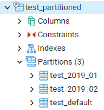
PostgreSQL Partition Table

Before version 10, it required a cumbersome method using inheritance, using triggers to connect the tables that inherit and receive. However, from version 10, it became simpler to use the parent-child relationship.

(1) Create partition PARENT

        
      
CREATE TABLE test.test_partitioned (
    dt        timestamp,
    message   text,
    code      int
) PARTITION BY RANGE(dt);
                  -- [RANGE | LIST | HASH]

Untitled

PARTITION BY RANGE(id): RANGE Partition based on the id range Example of partition_bound_spec setting: FOR VALUES FROM (1) to (1000)
PARTITION BY LIST(class): LIST Partition based on the class column Example of partition_bound_spec setting: FOR VALUES IN (‘G’, ‘V’)
PARTITION BY HASH(id): HASH Partition based on the id column Example of partition_bound_spec setting: FOR VALUES WITH (MODULUS 10, REMAINDER 5)
(2) Create CHILD table

        
      
CREATE TABLE test.test_2019_01
	PARTITION OF test.test_partitioned
	FOR VALUES
	FROM ('2019-01-01') to ('2019-02-01');

CREATE TABLE test.test_2019_02
	PARTITION OF test.test_partitioned
	FOR VALUES
	FROM ('2019-02-01') to ('2019-03-01');

CREATE TABLE test.test_default
	PARTITION OF test.test_partitioned
	DEFAULT;

Untitled

(3) Insert data

        
      
INSERT INTO test.test_partitioned VALUES ('2019-01-10', 'message...', 10);

(4) Delete partition

        
      
ALTER TABLE test.test_partitioned DETACH PARTITION test.test_2019_02;

💡 [Oracle]> [PostgreSQL[1][2](Official)(Inheritance-trigger method)]

3. `Replication method`

💡 Method of duplicating data across multiple nodes

4. `MapReduce`

💡 A software framework introduced by Google in 2004 for distributed parallel computing, designed to handle large-scale data processing. It consists of Map and Reduce processes:
Input (Data Input)
→ Splitting (Breaking down data and storing it in HDFS)
→ Mapping
→ Shuffling (Transferring data from Map function to Reduce function for aggregation of results from Map functions)
→ Reducing (Combining all values to extract the desired result)
→ Final Result - This process is followed for large-scale data processing.
[Source]

5. `Concurrency`

💡 Support for simultaneous data manipulation

6. `Durability`

💡 Support for persistent data generation

7. `In-Memory Features`

💡 Option to store some or all structures only in memory

8. `User Concepts`

💡 Access control

3. Installation

Install PostgreSQL

🔰 Files Installed Inside the PostgreSQL Data Directory

base: pg_default tablespace, stores data for each database in separate directories.
global: pg_global tablespace, manages data at the cluster level.
pg_hba.conf: Manages connections to PostgreSQL.
pg_log: Directory for log files.
pg_tblspc: User tablespace, creates symbolic links to tablespace directories.
postgresql.auto.conf: Records modifications to parameters made with the ALTER SYSTEM command.
postgresql.conf: Primary configuration file.

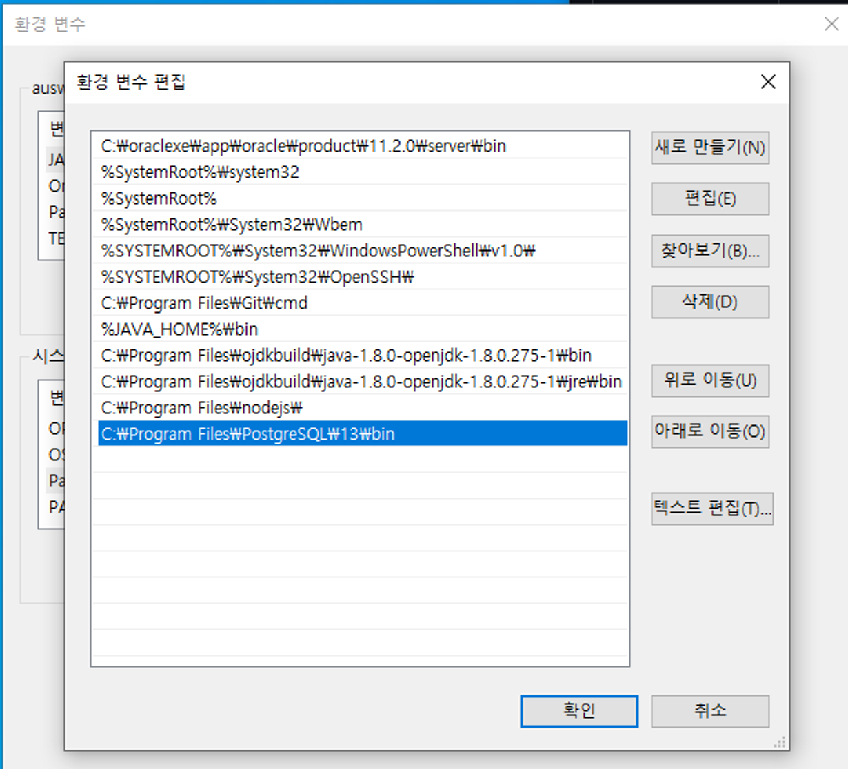
4. Environment Variable Configuration

Control Panel > System > Advanced System Settings > Environment Variables > System Variables > Edit Path

Untitled

5. Connection

SQL Shell (psql)

Command Prompt

        
  $ psql -U (postgres_name) // Connect
  $ psql --version // Check version

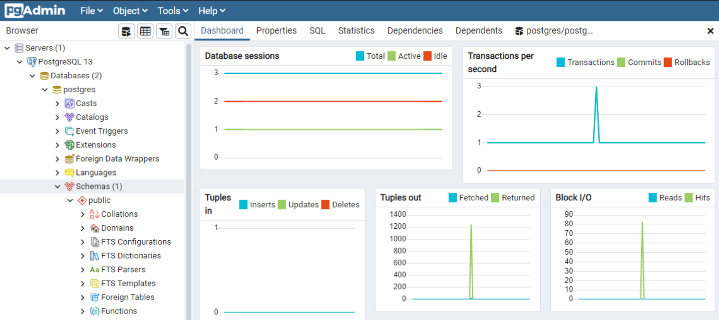
pgAdmin4 (Dedicated GUI tool)

Untitled

6. CRUD

Command	Description	Example
\q	Exit psql	-
\l	List databases	-
\c	Connect to a database	\c [dbName]
\e	Use an external editor	-
\dt	List tables in the current database	-
\db	List tablespaces	-

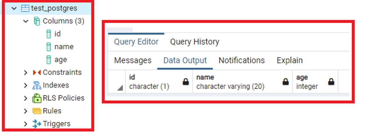
1) CREATE | `CREATE TABLE [tb_name] ([column_name] [data_type], ...);`

Untitled

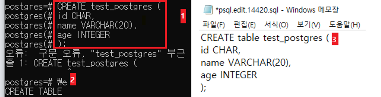
Enter the following commands in SQL shell *If there are syntax errors, an error message will be displayed
Enter the command \e
Modify the query in an external editor and save it

Untitled

        
      
-- Created after copying existing table (column and record data copied)
CREATE TABLE [new_table_name] AS
	SELECT * FROM [old_table_name]

        
      
-- Example
SELECT * FROM AddressBook;
// Result
id |  name  |                             attributes
----+--------+---------------------------------------------------------------------
  1 | 김가가 | "age"=>"38", "email"=>"111@aaa.co.kr", "telephone"=>"010-1111-1111"
  2 | 김나나 | "age"=>"29", "email"=>"222@bbb.co.kr", "telephone"=>"N/A"
(2 rows)

CREATE TABLE book AS SELECT * FROM AddressBook;
SELECT * FROM book;
// 결과
id |  name  |                             attributes
----+--------+---------------------------------------------------------------------
  1 | 김가가 | "age"=>"38", "email"=>"111@aaa.co.kr", "telephone"=>"010-1111-1111"
  2 | 김나나 | "age"=>"29", "email"=>"222@bbb.co.kr", "telephone"=>"N/A"
(2 rows)

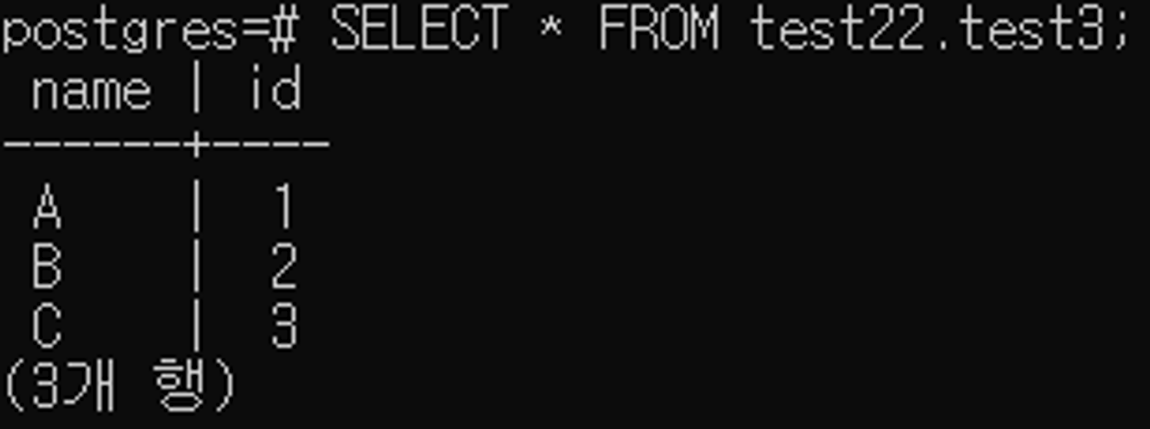
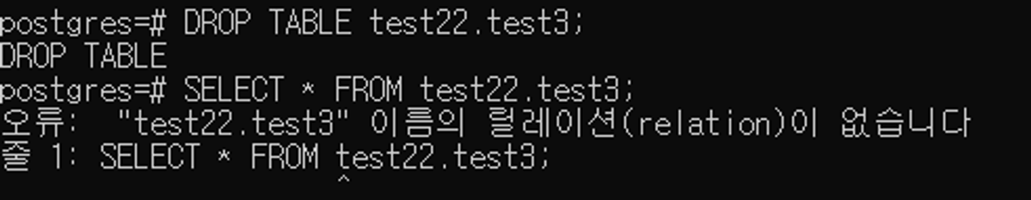
2) SELECT | `SELECT * FROM "[schema_name]".[tb_name];`

Untitled

3) INSERT & UPDATE

        
      
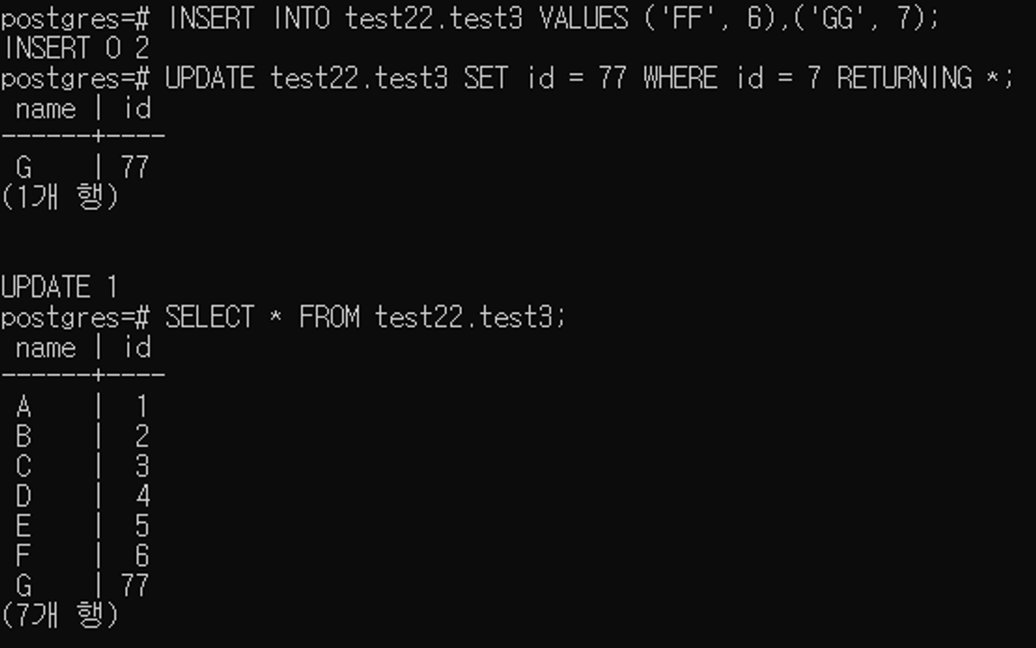
INSERT INTO [tb_name] ([column]) VALUES ([values]);
-- Add multiple
INSERT INTO book VALUES (1, 2, 3), (4, 5, 6), ..., (7, 8, 9);

UPDATE [tb_name] SET [column] = [values] WHERE [condition] [RETURNING *];
-- RETURNING * : View modified information immediately

Untitled

4) DELETE | `DROP TABLE [tb_name]`

Untitled

7. Data Types

Data Type	Alias	Description	Size
bigint	int8	Signed 8-byte integer
bigserial	serial8	Autoincrementing 8-byte integer
bit [ (n) ]		Fixed-length bit string
bit varying [ (n) ]	varbit	Variable-length bit string
boolean	bool	Logical Boolean (true/false)
box		Rectangular box on a plane
bytea		Binary data (“byte array”)
character [ (n) ]	char [ (n) ]	Fixed-length character string
character varying [ (n) ]	varchar [ (n) ]	Variable-length character string
cidr		IPv4 or IPv6 network address
circle		Circle on a plane
date		Calendar date (year, month, day)	4
double precision	float8	Double precision floating-point (8 bytes)	8
inet		IPv4 or IPv6 host address
integer	int, int4, numeric(n)[numeric with a limit on the number of digits]	Signed 4-byte integer	4
interval [ fields ] [ (p) ]		Time interval
line		Infinite line on a plane
lseg		Line segment on a plane
macaddr		MAC (Media Access Control) address
money		Currency amount
numeric [ (p, s) ]	decimal [ (p, s) ]	User-specified precision, exact numeric type	Variable
path		Geometric path on a plane
point		Geometric point on a plane
polygon		Closed geometric path on a plane
real	float4	Single precision floating-point (4 bytes)	4
serial	serial4	Autoincrementing 4-byte integer	4
smallint	int2	Signed 2-byte integer
text		Variable-length character string
time [ (p) ] [ without time zone ]		Time of day (no time zone)	8
time [ (p) ] with time zone	timetz	Time of day with time zone	12
timestamp [ (p) ] [ without time zone ]		Date and time (no time zone)	8
timestamp [ (p) ] with time zone	timestamptz	Date and time with time zone (GMT+9)	8
tsquery		Text search query
tsvector		Text search document
txid_snapshot		User-level transaction ID snapshot
uuid		Universally unique identifier
xml		XML data

timestamp [ (p) ] with time zone

        
-- Print time zone information
SHOW TIMEZONE;

-- Time setting
SET TIMEZONE = 'America/Los_Angeles';

Other data types

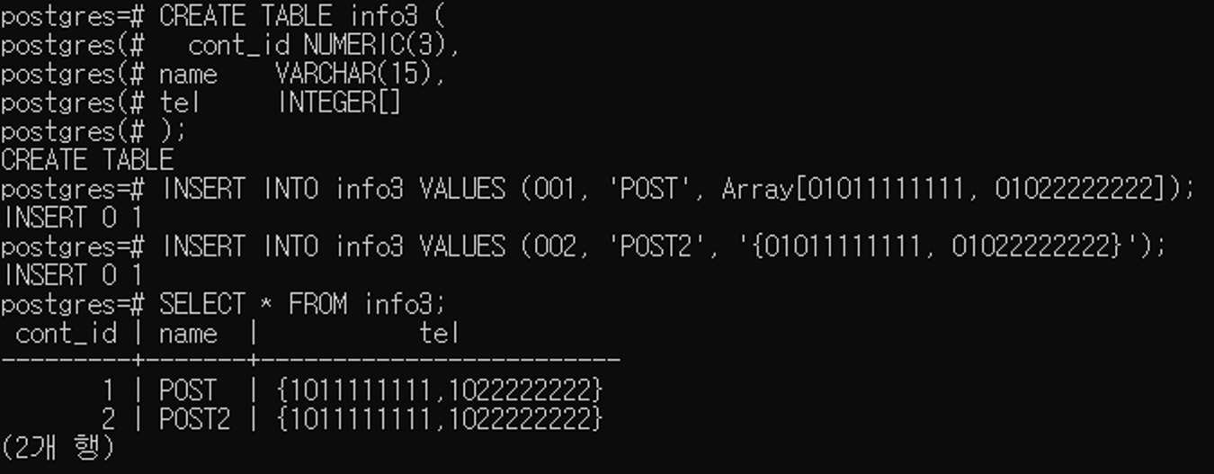
🔰 Array type : Array[]

        
      
CREATE TABLE info3 (
  cont_id NUMERIC(3),
  name    VARCHAR(15),
  tel     INTEGER[]
);

INSERT INTO info3 VALUES (001, 'POST', Array[01011111111, 01022222222]);
INSERT INTO info3 VALUES (002, 'POST2', '{01011111111, 01022222222}');

Untitled

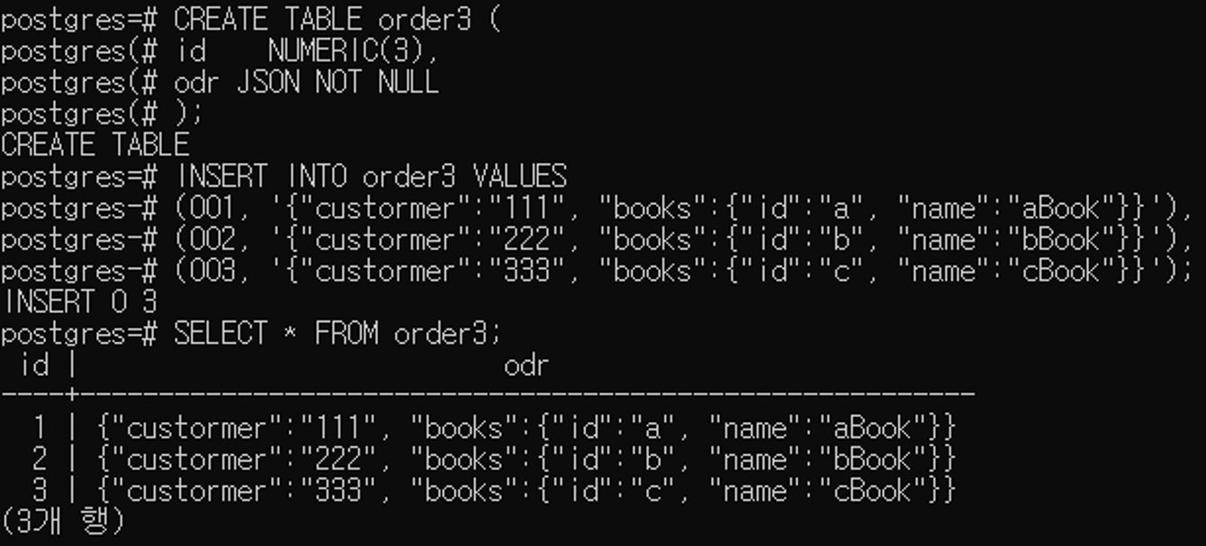
🔰 JSON type : JOSN / JSONB

        
SELECT '{"bar": "baz",           "balanc   e": 7.77, "active":false}'::json;
// "{""bar"": ""baz"",           ""balanc   e"": 7.77, ""active"":false}"

SELECT '{"bar": "baz",            "balanc   e": 7.77, "active":false}'::jsonB;
// "{""bar"": ""baz"", ""active"": false, ""balanc   e"": 7.77}"

JSON stores values exactly as they are received. However, JSONB does not store them as is. It removes spaces between strings and does not guarantee the order of keys.

        
      
CREATE TABLE order3 (
  id    NUMERIC(3),
  odr   JSON NOT NULL
);

INSERT INTO order3 VALUES
  (001, '{"custormer":"111", "books":{"id":"a", "name":"aBook"}}'),
  (002, '{"custormer":"222", "books":{"id":"b", "name":"bBook"}}'),
  (003, '{"custormer":"333", "books":{"id":"c", "name":"cBook"}}');

Untitled

8. Uses

1) Operators and Functions

PostgreSQL	ORACLE
SELECT 1;	SELECT 1 FROM dual;
NEXTVAL.[sequence_name]	[sequence_name].NEXTVAL
CAST(expression AS target_data_type)	TO_CHAR, TO_NUMBER, etc., for type conversion
COALESCE(, ,...)	NVL(column, substitute_value)
NULLIF(, ,...)	NULLIF(, ,...)
now(), CURRENT_DATE, etc., for date and time functions	SYSDATE, SYSTIMESTAMP
CASE columns1 when val1 then result1 … else default END	DECODE(column1, val1, result1, …, default)
WITH RECURSIVE	CONNECT BY
TEXT(data_type)	CLOB

1. `SELECT 1;`

Inline view

An inline view refers to a subquery used in the FROM clause. When using an inline view, it is necessary to provide an alias.

        
      
SELECT *
FROM (
  SELECT '{
    "guid": "9c36adc1-7fb5-4d5b-83b4-90356a46061a",
    "name": "Angela Barton",
    "is_active": true,
    "company": "Magnafone",
    "address": "178 Howard Place, Gulf, Washington, 702",
    "registered": "2009-11-07T08:53:22 +08:00",
    "latitude": 19.793713,
    "longitude": 86.513373,
    "tags": [ "enim", "aliquip", "qui" ]
    }'::json
) AS test_table;

// Result
{
  "guid": "9c36adc1-7fb5-4d5b-83b4-90356a46061a",
  "name": "Angela Barton",
  "is_active": true,
  "company": "Magnafone",
  "address": "178 Howard Place, Gulf, Washington, 702",
  "registered": "2009-11-07T08:53:22 +08:00",
  "latitude": 19.793713,
  "longitude": 86.513373,
  "tags": [ "enim", "aliquip", "qui" ]
}
// Result(SHELL)
json
---------------------------------------------------------
{                                                       +
  "guid": "9c36adc1-7fb5-4d5b-83b4-90356a46061a",       +
  "name": "Angela Barton",                              +
  "is_active": true,                                    +
  "company": "Magnafone",                               +
  "address": "178 Howard Place, Gulf, Washington, 702", +
  "registered": "2009-11-07T08:53:22 +08:00",           +
  "latitude": 19.793713,                                +
  "longitude": 86.513373,                               +
  "tags": [ "enim", "aliquip", "qui" ]                  +
}
(1 row)

SELECT *
FROM (
  SELECT '{
      "guid": "9c36adc1-7fb5-4d5b-83b4-90356a46061a",
      "name": "Angela Barton",
      "is_active": true,
      "company": "Magnafone",
      "address": "178 Howard Place, Gulf, Washington, 702",
      "registered": "2009-11-07T08:53:22 +08:00",
      "latitude": 19.793713,
      "longitude": 86.513373,
      "tags": [ "enim", "aliquip", "qui" ]
    }'::json
);

// Result
ERROR: error:  In the FROM clause, a subquery must always have an alias.
LINE 2: FROM (
             ^
HINT:  example, FROM (SELECT ...) [AS] foo.

Single row subquery

        
      
SELECT address
  FROM test_table
WHERE phone = (SELECT phone FROM p_table WEHRE name = 'test_name');

2. `CAST(Expression AS Data type to change)`

        
      
SELECT CAST('3000' AS INTEGER); // 3000

SELECT CAST('2020-08-11' AS TEXT), CAST('2020-08-11' AS DATE);
// Result
text    |    date
------------+------------
 2020-08-11 | 2020-08-11
(1 row)

SELECT '00:15:00'::TIME; // 00:15:00

3. `COALESCE(<parameter1>, <parameter2>,...)`

💡 Difference with Oracle

Oracle: NVL(hire_date, SYSDATE) - Implicit type conversion occurs if types do not match
PostgreSQL: COALESCE(hire_date, SYSDATE) - Error if column types do not match (constants are OK)

        
SELECT COALESCE(null, null, null, 'empty value') AS column1; // empty value
SELECT COALESCE(null, 1); // 1

        
      
postgres=# SELECT * FROM test;
// Result
 id
----
  1
  2
  3
  4
  5
 null
(6 rows)

postgres=# SELECT COALESCE(id, 0) AS col1 FROM test;
// Result
col1
------
    1
    2
    3
    4
    5
    0
(6 rows)

4. `NULLIF(<parameter1>, <parameter2>,...)`

💡 Returns NULL if equals , Returns if does not equal .
1 2 SELECT NULLIF(20, 20); // NULL SELECT NULLIF(22, 23); // 22

5. `now(), CURRENT_DATE, and other Date/Time Functions`

Function	Description	Example
CURRENT_DATE	Returns current date	SELECT CURRENT_DATE;
CURRENT_TIME	Returns current time with time zone	SELECT CURRENT_TIME(2);
CURRENT_TIMESTAMP	Returns current date and time with time zone	SELECT CURRENT_TIMESTAMP(2);
LOCALTIME	Returns current time	SELECT LOCALTIME(2);
LOCALTIMESTAMP	Returns current date and time	SELECT LOCALTIMESTAMP;
age()	Returns the difference between current date and date	SELECT age(timestamp ‘2020-03-01’);
EXTRACT	Extracts specific information from date and time data types	SELECT EXTRACT(MONTH FROM TIMESTAMP ‘2020-09-20’); // Returns 9 for September
date_part()	Similar to EXTRACT, but the field value is received as a string	SELECT date_part(‘month’, now()); // Returns 3 for March
date_trunc()	Removes unnecessary date information	SELECT date_trunc(‘month’, now()); // Returns “2021-03-01 00:00:00+09” // (At the time of execution: 2021-03-04)

EXTRACT field values

CENTURY	Century
QUARTER	Quarter
YEAR	Year
MONTH	Month
DAY	Day
HOUR	Hour
MINUTE	Minute
SECOND	Second
ISODOW	ISO day of the week (Monday(1) to Sunday(7))
DOW	Day of the week (Sunday(0) to Saturday(6))
TIMEZONE	Timezone

6. `WITH RECURSIVE`

        
      
-- PostgreSQL
with recursive VIEWNAME as(
    -- Initial SQL
    -- union all(or union)
    -- Recursive SQL (+ condition to stop recursion)
)select * from 뷰명;

with recursive VIEWNAME as(
    SELECT 1 AS num
    UNION ALL
    SELECT num + 1 FROM VIEWNAME WHERE num < 10
)select * from VIEWNAME;

-- Oracle
SELECT [columns]...
	FROM [table]
WHERE [condition]
	START WITH [top-level condition]
CONNECT BY [NOCYCLE] [PRIOR hierarchical condition];

SELECT
	DEPT_NAME,
	DEP_CD,
	PARENT_CD,
	LEVEL
FROM DEP
	START WITH PARENT_CD IS NULL -- Set the top-level node
CONNECT BY PRIOR DEP_CD = PARENT_CD; -- Connect parent and child nodes

7. `TEXT(Data Type)`

💡 What is CLOB?

According to the CUBRID manual, it is described as follows: In simple terms, it is a data type for storing large-sized data in external files.

Used for storing string data externally in the database.

The maximum length of CLOB data is determined by the file size that can be generated in external storage.

The CLOB type represents input and output values as string types in SQL statements. In other words, it is compatible with CHAR(n), VARCHAR(n), NCHAR(n), and NCHAR VARYING(n) types. However, only explicit type conversion is allowed, and in case of different data lengths, the maximum length is adjusted to the smaller type by truncation.

When converting a CLOB type value to a string, the converted data cannot exceed 1GB. Conversely, when converting a string to a CLOB type, the converted data cannot exceed the maximum file size provided by the CLOB storage.

Additional Operators and Functions

Array Functions

Operator/Function	Description	Example	Expected Result
array_append()	- Append an element to the end of an array. - `1 \|\| ARRAY[2, 3] = {1, 2, 3}`	`array_append(ARRAY[1, 2], 3)`	Array
array_prepend()	Prepend an element to the beginning of an array	`array_prepend(1, ARRAY[2, 3])`	Array
array_remove()	Remove a specific element from an array	`array_remove(array, element)`	Array
array_replace()	Replace a specific element in an array with another element	`array_replace(array, element1, element2)`	Array
array_cat()	Concatenate two arrays	`array_cat(array1, array2)`	Array
<@ or @>	Containment operator	`ARRAY[1, 2, 3] @> ARRAY[1, 3]`	boolean,NULL

JSON and JSONB Functions

Operator/Function	Description	Example	Expected Result
->	Retrieve a value from a JSON object using a key or index from a JSON array	`'{"a":"a1", "b":"b1", "c":"c1"}' :: json -> 'a'` `'[{"a":"a1"}, {"b": "b1"}, {"c":"c1"}]' :: json -> 1`	JSON
-»	Retrieve data from JSON objects or JSON arrays as text	`'{"a":{"a":"c"}, "b":{"b":"d"}}' :: json ->> 'a'`	TEXT
#>	Retrieve the value at a specific path	`'{"a":{"b":{"c":"d"}}}' :: json #> '{"a", "b", "c"}'`	JSON
#»	Retrieve the value at a specific path as TEXT data type	`'{"a":[{"b":"d"}, {"c":"f"}]}' :: json #>> '{"a", 0, "b"}'`	TEXT
?	Determine if a specified string exists as a key in JSONB	`'{"a":0, "b":1}' :: jsonb ? 'a'`	boolean,NULL
`?\|`	Determine if one or more elements in an array exist as keys in JSONB	`'{"a":0, "b":1, "c":2}' :: jsonb ?\| array['b', 'd']`	boolean,NULL
?&	Determine if all elements in an array exist as keys in JSONB	`'{"a":0, "b":1, "c":2}' :: jsonb ?& array['b', 'd']`	boolean,NULL
-	- Remove one or more elements from a JSONB object. - Remove the element at the specified index from a JSONB array	`'{"a":0, "b":1}' :: jsonb - 'b'`	JSONB

JSON and JSONB Functions

Operator/Function	Description	Example	Expected Result
json_build_object()	JSON object creation function	`json_build_object("<key1>", "<value1>", "<key2>", "<value2>", ...)`	JSON
json_build_array()	Function to create a JSON-formatted JSON array	`json_build_array("<element1>", "<element2>", "<element3>", ...)`	JSON
json_array_length()	Number of elements in a JSON array	`json_array_length(<JSON>)`	INTEGER
json_each()	Organize key-value pairs as columns in the JSON data type	`json_each(<JSON object>)`	JSON
json_array_elements()	Retrieve elements from a JSON array as columns	`json_array_elements(<JSON array>)`	JSON
json_agg()	Aggregate values into a JSON array, including null values	See details	-
jsonb_agg()	Aggregate values into a JSONB array, including null values	See details	-
json_object_agg(name, value)	Aggregate name-value pairs into a JSON object (value includes null, name excludes null)	See details	-
jsonb_object_agg(name, value)	Aggregate name-value pairs into a JSONB object (value includes null, name excludes null)	See details	-

1. `- >`

        
SELECT '{"a":"a1", "b":"b1", "c":"c1"}' :: json -> 'a'; // 'a1'
SELECT '[{"a":"a1"}, {"b": "b1"}, {"c":"c1"}]' :: json -> 1; // "{"b": "b1"}"

2. `- >>`

        
      
SELECT
	'{"a":{"a":"c"}, "b":{"b":"d"}}' :: json ->> 'a' // "{"a":"c"}"
;

3. `# >`

        
      
SELECT
	'{"a":{"b":{"c":"d"}}}' :: json #> '{"a", "b", "c"}' // "d"
;

4. `# >>`

        
      
SELECT
	'{"a":[{"b":"d"}, {"c":"f"}]}' :: json #>> '{"a", 0, "b"}' // "d"
;

5. `-`

        
      
SELECT
	'{"a":0, "b":1}' :: jsonb - 'b' // "{"a": 0}"
;

6. `json_build_object()`

        
      
SELECT
	json_build_object('a', 1, 'b', 2) // "{"a" : 1, "b" : 2}"
;

7. `json_build_array()`

        
      
SELECT
	json_build_array('a', 1, 'b', 2) // "["a", 1, "b", 2]"
;

8. `json_array_length()`

        
      
SELECT
	json_array_length('["a", 1, "b", 2]') // 4
;

9. `json_each()`

        
      
SELECT * FROM
	json_each('{"JAMES":"HANDSOME", "JASON":"UGLY"}')
;

// Result
key  |   value
-------+------------
 JAMES | "HANDSOME"
 JASON | "UGLY"
(2 rows)

10. `json_array_elements()`

        
      
SELECT * FROM
	json_array_elements('[1, "a", {"b":"c"}, ["d", 2, 3]]')
;

// Result
value
-------------
 1
 "a"
 {"b":"c"}
 ["d", 2, 3]
(4 rows)

11. `json_agg()`

        
      
SELECT * FROM order3;

// Result
id |                           odr
----+---------------------------------------------------------
  1 | {"custormer":"111", "books":{"id":"a", "name":"aBook"}}
  2 | {"custormer":"222", "books":{"id":"b", "name":"bBook"}}
  3 | {"custormer":"333", "books":{"id":"c", "name":"cBook"}}
(3 rows)

        
      
-- Designate the id column as a group and aggregate data in the odr column

SELECT id, json_agg(odr) FROM order3 GROUP BY 1;

// Result
id |                         json_agg
----+-----------------------------------------------------------
  3 | [{"custormer":"333", "books":{"id":"c", "name":"cBook"}}]
  1 | [{"custormer":"111", "books":{"id":"a", "name":"aBook"}}]
  2 | [{"custormer":"222", "books":{"id":"b", "name":"bBook"}}]
(3 rows)

12. `jsonb_agg()`

        
      
SELECT * FROM order3;

// Result
id |                           odr
----+---------------------------------------------------------
  1 | {"custormer":"111", "books":{"id":"a", "name":"aBook"}}
  2 | {"custormer":"222", "books":{"id":"b", "name":"bBook"}}
  3 | {"custormer":"333", "books":{"id":"c", "name":"cBook"}}
(3 rows)

        
      
-- Designate the id column as a group and aggregate data in the odr column

SELECT id, jsonb_agg(odr) FROM order3 GROUP BY 1;

// Result(JSONB)
id |                           jsonb_agg
----+---------------------------------------------------------------
  3 | [{"books": {"id": "c", "name": "cBook"}, "custormer": "333"}]
  1 | [{"books": {"id": "a", "name": "aBook"}, "custormer": "111"}]
  2 | [{"books": {"id": "b", "name": "bBook"}, "custormer": "222"}]
(3 rows)

// Result(JSON)
id |                         json_agg
----+-----------------------------------------------------------
  3 | [{"custormer":"333", "books":{"id":"c", "name":"cBook"}}]
  1 | [{"custormer":"111", "books":{"id":"a", "name":"aBook"}}]
  2 | [{"custormer":"222", "books":{"id":"b", "name":"bBook"}}]
(3 rows)

13. `json_object_agg(name, value)`

        
      
SELECT * FROM order3;

// Result
id |                           odr
----+---------------------------------------------------------
  1 | {"custormer":"111", "books":{"id":"a", "name":"aBook"}}
  2 | {"custormer":"222", "books":{"id":"b", "name":"bBook"}}
  3 | {"custormer":"333", "books":{"id":"c", "name":"cBook"}}
(3 rows)

        
      
SELECT
	json_object_agg(id, odr)
FROM order3
;

// Print Result
"{
 ""1"" : {""custormer"":""111"", ""books"":{""id"":""a"", ""name"":""aBook""}},
 ""2"" : {""custormer"":""222"", ""books"":{""id"":""b"", ""name"":""bBook""}},
 ""3"" : {""custormer"":""333"", ""books"":{""id"":""c"", ""name"":""cBook""}}
 }"

14. `jsonb_object_agg(name, value)`

        
      
SELECT * FROM order3;

// Result
id |                           odr
----+---------------------------------------------------------
  1 | {"custormer":"111", "books":{"id":"a", "name":"aBook"}}
  2 | {"custormer":"222", "books":{"id":"b", "name":"bBook"}}
  3 | {"custormer":"333", "books":{"id":"c", "name":"cBook"}}
(3 rows)

        
      
SELECT
	jsonb_object_agg(id, odr)
FROM order3
;

// Print Result(JSONB)
"{
 ""1"": {""books"": {""id"": ""a"", ""name"": ""aBook""}, ""custormer"": ""111""},
 ""2"": {""books"": {""id"": ""b"", ""name"": ""bBook""}, ""custormer"": ""222""},
 ""3"": {""books"": {""id"": ""c"", ""name"": ""cBook""}, ""custormer"": ""333""}
 }"

// Print Result(JSON)
"{
 ""1"" : {""custormer"":""111"", ""books"":{""id"":""a"", ""name"":""aBook""}},
 ""2"" : {""custormer"":""222"", ""books"":{""id"":""b"", ""name"":""bBook""}},
 ""3"" : {""custormer"":""333"", ""books"":{""id"":""c"", ""name"":""cBook""}}
 }"

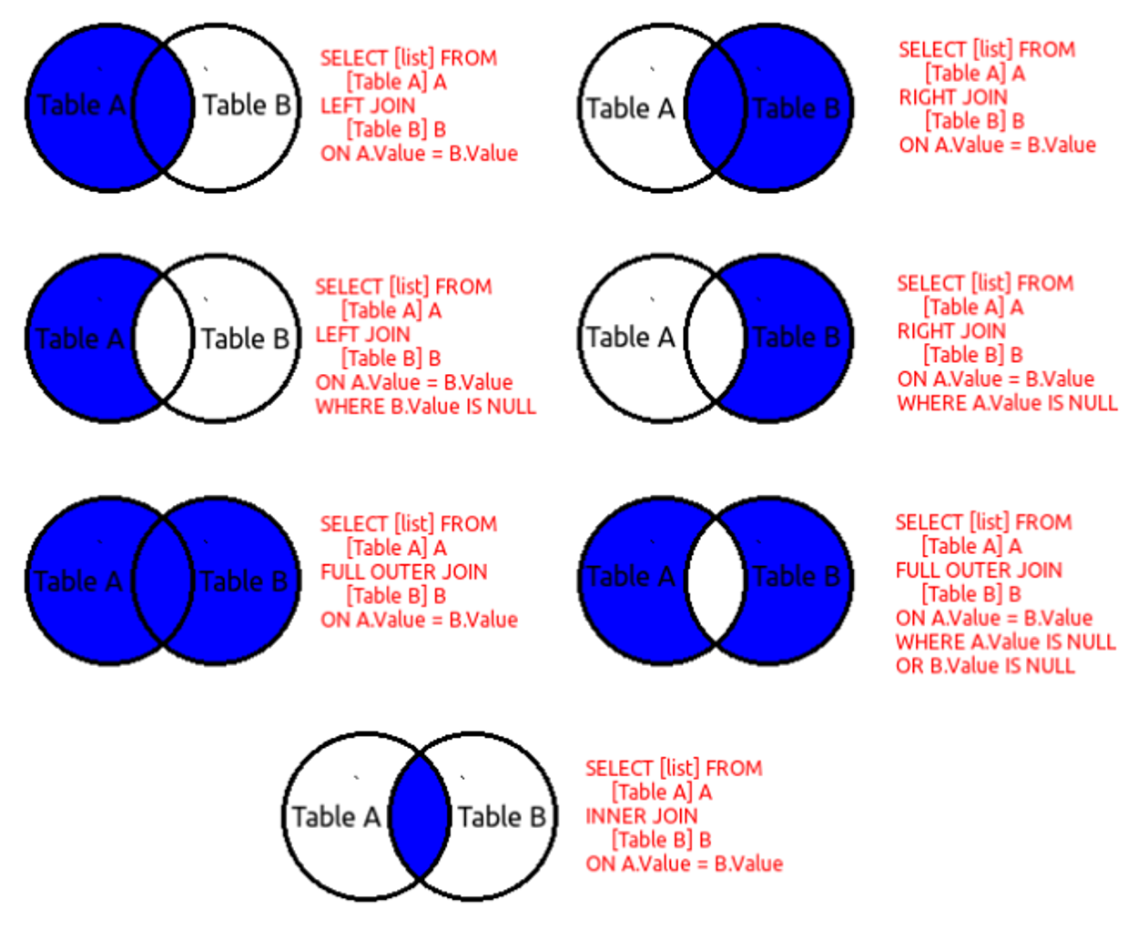
2) Join

Untitled

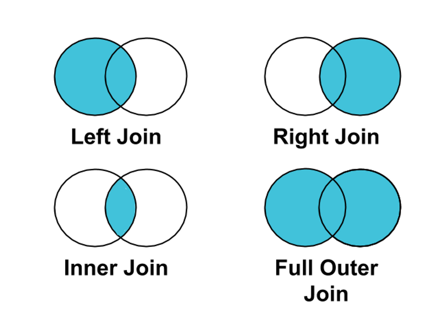
INNER JOIN

The results in the following examples are all the same, and there is no difference in performance.

        
      
SELECT
	pg_database.dattablespace AS dtspcoid, datname, pg_database.oid,
	pg_tablespace.oid AS spcoid, spcname, spcowner
FROM pg_database, pg_tablespace WHERE pg_database.dattablespace = pg_tablespace.oid;

// Result
dtspcoid |  datname  |  oid  | spcoid |   spcname    | spcowner
----------+-----------+-------+--------+--------------+----------
     1663 | postgres  | 13442 |   1663 | pg_default   |       10
     1663 | test      | 16394 |   1663 | pg_default   |       10
     1663 | template1 |     1 |   1663 | pg_default   |       10
     1663 | template0 | 13441 |   1663 | pg_default   |       10
    16735 | mytable   | 16736 |  16735 | mytablespace |       10
    16746 | mytest    | 16747 |  16746 | tbs1         |       10
    16748 | mytest2   | 16749 |  16748 | tbs2         |       10
     1663 | testdb    | 16757 |   1663 | pg_default   |       10
     1663 | newuserdb | 16774 |   1663 | pg_default   |       10
(9 rows)

SELECT
	pg_database.dattablespace AS dtspcoid, datname, pg_database.oid,
	pg_tablespace.oid AS spcoid, spcname, spcowner
FROM pg_database INNER JOIN pg_tablespace ON pg_database.dattablespace = pg_tablespace.oid;

// Result
dtspcoid |  datname  |  oid  | spcoid |   spcname    | spcowner
----------+-----------+-------+--------+--------------+----------
     1663 | postgres  | 13442 |   1663 | pg_default   |       10
     1663 | test      | 16394 |   1663 | pg_default   |       10
     1663 | template1 |     1 |   1663 | pg_default   |       10
     1663 | template0 | 13441 |   1663 | pg_default   |       10
    16735 | mytable   | 16736 |  16735 | mytablespace |       10
    16746 | mytest    | 16747 |  16746 | tbs1         |       10
    16748 | mytest2   | 16749 |  16748 | tbs2         |       10
     1663 | testdb    | 16757 |   1663 | pg_default   |       10
     1663 | newuserdb | 16774 |   1663 | pg_default   |       10
(9 rows)

SELECT
	pg_database.dattablespace AS dtspcoid, datname, pg_database.oid,
	pg_tablespace.oid AS spcoid, spcname, spcowner
FROM (
	pg_database JOIN pg_tablespace ON pg_database.dattablespace = pg_tablespace.oid
);

// Result
dtspcoid |  datname  |  oid  | spcoid |   spcname    | spcowner
----------+-----------+-------+--------+--------------+----------
     1663 | postgres  | 13442 |   1663 | pg_default   |       10
     1663 | test      | 16394 |   1663 | pg_default   |       10
     1663 | template1 |     1 |   1663 | pg_default   |       10
     1663 | template0 | 13441 |   1663 | pg_default   |       10
    16735 | mytable   | 16736 |  16735 | mytablespace |       10
    16746 | mytest    | 16747 |  16746 | tbs1         |       10
    16748 | mytest2   | 16749 |  16748 | tbs2         |       10
     1663 | testdb    | 16757 |   1663 | pg_default   |       10
     1663 | newuserdb | 16774 |   1663 | pg_default   |       10
(9 rows)

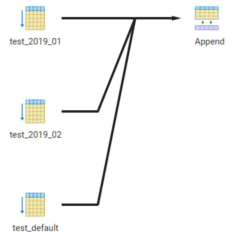
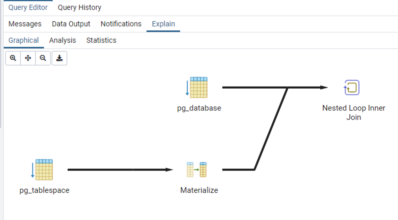
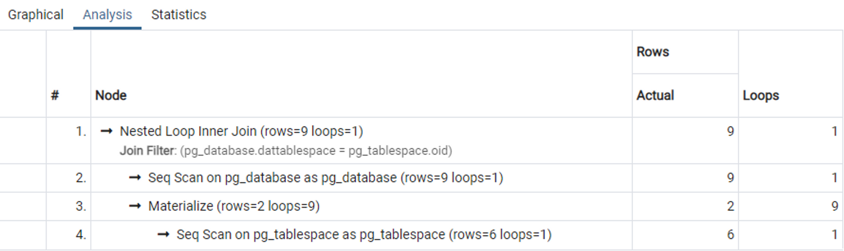
Checking the join structure (visually)

🔰 SHELL

        
      
EXPLAIN ([ANALYZE]) -- Added
SELECT
	pg_database.dattablespace AS dtspcoid, datname, pg_database.oid,
	pg_tablespace.oid AS spcoid, spcname, spcowner
FROM (
	pg_database JOIN pg_tablespace ON pg_database.dattablespace = pg_tablespace.oid
);

// Result
QUERY PLAN
--------------------------------------------------------------------------
 Nested Loop  (cost=0.00..2.09 rows=2 width=144)
   Join Filter: (pg_database.dattablespace = pg_tablespace.oid)
   ->  Seq Scan on pg_database  (cost=0.00..1.02 rows=2 width=72)
   ->  Materialize  (cost=0.00..1.03 rows=2 width=72)
         ->  Seq Scan on pg_tablespace  (cost=0.00..1.02 rows=2 width=72)
(5 rows)

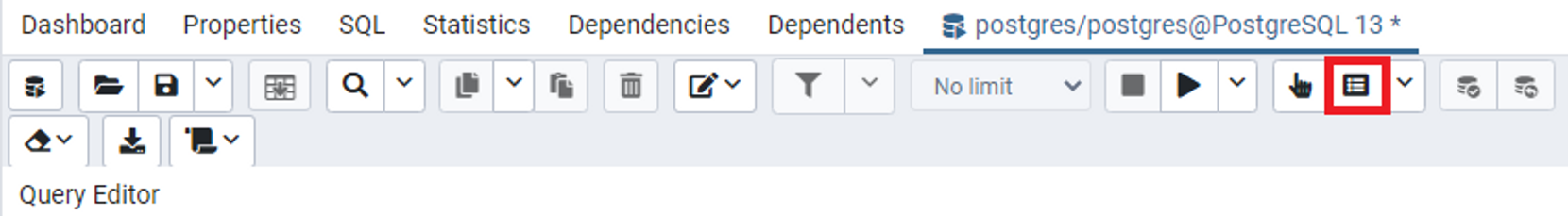
🔰 PgAdmin

Untitled

LEFT OUTER JOIN

The command retrieves information based on the table mentioned first, connecting it with the table mentioned later. If there is no connected information, it outputs NULL values.

        
      
SELECT
	pg_tablespace.oid AS spcoid,
	spcname,
	spcowner
FROM pg_tablespace;

// Result(6 rows)
spcoid |   spcname    | spcowner
--------+--------------+----------
   1663 | pg_default   |       10
   1664 | pg_global    |       10
  16730 | test         |       10
  16735 | mytablespace |       10
  16746 | tbs1         |       10
  16748 | tbs2         |       10

        
      
SELECT
	pg_database.dattablespace AS dtspcoid,
	datname, pg_database.oid
FROM pg_database;

// Result(9 rows)
dtspcoid |  datname  |  oid
----------+-----------+-------
     1663 | postgres  | 13442
     1663 | test      | 16394
     1663 | template1 |     1
     1663 | template0 | 13441
    16735 | mytable   | 16736
    16746 | mytest    | 16747
    16748 | mytest2   | 16749
     1663 | testdb    | 16757
     1663 | newuserdb | 16774

✅ The information from the pg_tablespace table is matched with the information from the pg_database table based on certain conditions. Columns in pg_tablespace without matching values are output as NULL.

        
      
SELECT
	pg_database.dattablespace AS dtspcoid, datname, pg_database.oid,
	pg_tablespace.oid AS spcoid, spcname, spcowner
FROM pg_tablespace LEFT JOIN pg_database ON pg_database.dattablespace = pg_tablespace.oid;

// Result(11 rows)
dtspcoid |  datname  |  oid  | spcoid |   spcname    | spcowner
----------+-----------+-------+--------+--------------+----------
     1663 | postgres  | 13442 |   1663 | pg_default   |       10
     1663 | test      | 16394 |   1663 | pg_default   |       10
     1663 | template1 |     1 |   1663 | pg_default   |       10
     1663 | template0 | 13441 |   1663 | pg_default   |       10
    16735 | mytable   | 16736 |  16735 | mytablespace |       10
    16746 | mytest    | 16747 |  16746 | tbs1         |       10
    16748 | mytest2   | 16749 |  16748 | tbs2         |       10
     1663 | testdb    | 16757 |   1663 | pg_default   |       10
     1663 | newuserdb | 16774 |   1663 | pg_default   |       10
   (NULL) |  (NULL)   | (NULL)|  16730 | test         |       10
   (NULL) |  (NULL)   | (NULL)|   1664 | pg_global    |       10

RIGHT OUTER JOIN

Retrieve information from the table specified after the command, based on the conditions, and match it with the table specified before the command. If there is no matching information, display NULL values.

✅ Based on the pg_database table, retrieve information from pg_tablespace where the conditions are met, and display NULL values for columns in pg_tablespace where there is no matching value. In this case, since there are no instances without matching values, all columns from pg_tablespace are displayed with their corresponding matched values from the pg_database table.

        
      
SELECT
	pg_database.dattablespace AS dtspcoid, datname, pg_database.oid,
	pg_tablespace.oid AS spcoid, spcname, spcowner
FROM pg_tablespace RIGHT JOIN pg_database ON pg_database.dattablespace = pg_tablespace.oid;

// Result(9 rows)
dtspcoid |  datname  |  oid  | spcoid |   spcname    | spcowner
----------+-----------+-------+--------+--------------+----------
     1663 | postgres  | 13442 |   1663 | pg_default   |       10
     1663 | test      | 16394 |   1663 | pg_default   |       10
     1663 | template1 |     1 |   1663 | pg_default   |       10
     1663 | template0 | 13441 |   1663 | pg_default   |       10
    16735 | mytable   | 16736 |  16735 | mytablespace |       10
    16746 | mytest    | 16747 |  16746 | tbs1         |       10
    16748 | mytest2   | 16749 |  16748 | tbs2         |       10
     1663 | testdb    | 16757 |   1663 | pg_default   |       10
     1663 | newuserdb | 16774 |   1663 | pg_default   |       10

FULL OUTER JOIN

Connect the rows that are linked and display them together. For the rows that are not linked, output the information for the unlinked parts with NULL values.

        
      
SELECT
	pg_database.dattablespace AS dtspcoid, datname, pg_database.oid,
	pg_tablespace.oid AS spcoid, spcname, spcowner
FROM pg_tablespace FULL OUTER JOIN pg_database ON pg_database.dattablespace = pg_tablespace.oid;

// Result(11 rows)
dtspcoid |  datname  |  oid  | spcoid |   spcname    | spcowner
----------+-----------+-------+--------+--------------+----------
     1663 | postgres  | 13442 |   1663 | pg_default   |       10
     1663 | test      | 16394 |   1663 | pg_default   |       10
     1663 | template1 |     1 |   1663 | pg_default   |       10
     1663 | template0 | 13441 |   1663 | pg_default   |       10
    16735 | mytable   | 16736 |  16735 | mytablespace |       10
    16746 | mytest    | 16747 |  16746 | tbs1         |       10
    16748 | mytest2   | 16749 |  16748 | tbs2         |       10
     1663 | testdb    | 16757 |   1663 | pg_default   |       10
     1663 | newuserdb | 16774 |   1663 | pg_default   |       10
   (NULL) |  (NULL)   | (NULL)|  16730 | test         |       10
   (NULL) |  (NULL)   | (NULL)|   1664 | pg_global    |       10

3) Index

Feature

When executing a query without an index, it is necessary to individually retrieve all rows. Indexing makes query operations very efficient.
If new rows are frequently inserted or removed with an existing index, performance degradation may occur because the index needs to be updated each time.
Simple indexes can be used when querying a specific column, while composite indexes are efficient when querying multiple columns.
The order of columns is crucial in composite indexes.

B-Tree Index

Untitled

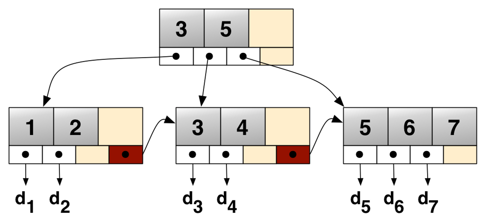
A tree structure where the maximum number of child nodes is greater than 2.
All keys in each node are sorted, and parent-child nodes are connected.
Connected nodes between parent and child should contain only values between the two key values.
In this sorted state, you can search by comparing values by traversing nodes.
Automatically generated index when creating a PK key.

💡 Drawback: If the number of child nodes increases or, conversely, if a node contains few key values, the search efficiency may decrease. Therefore, it is necessary to organize the index according to rules that ensure the fewest number of queries during the search (balance adjustment).

        
      
// B-tree Index Creation: The default is B-Tree even if no options are specified.
-- `Single-column index`: a method where an index column has a single type of value (e.g., PK).
CREATE INDEX [index_name] ON [table_name] USING btree ([column_name]);
-- `Composite-column index` : a method where two or more columns have multiple values.
-- (You need to decide which of the two column values to prioritize)
CREATE INDEX [index_name]
	ON [table_name] ([column_name1] [ASC|DESC], [column_name2] [ASC|DESC]);
-- `Partial Index` : Creating an index only for values that meet specific conditions rather than all values in a column.
CREATE INDEX [index_name] ON [table_name]([column_name]) WHERE [condition]
-- ex) CREATE INDEX male_index ON male(isHandsome) WHERE isHandsome is not null;

        
      
// Check the created index
-- along with its creation statement
SELECT * FROM pg_indexes WHERE tablename='[table_name]';
-- Check the size of the index table
\di+

// Modify an index
ALTER INDEX <index_name> RENAME TO <new_index_name>;

// Drop a created index
DROP INDEX <index_name>;

Hash Index

A B-Tree structure is created based on values transformed into a smaller size through a hash function.
The index size is much smaller compared to using only the B-Tree structure, making it efficient in terms of memory caching and search speed.

💡 Drawback: Since the original values are transformed through a hash function, it is not possible to compare the size between indexed column values. Sorting and comparison operations are not possible with index usage. Only equality comparisons are possible using the equal sign. Therefore, it is not a commonly used indexing method.

        
// Create Hash Index
CREATE INDEX [index_name] ON [table_name] UNING HASH([column_name]);

GIN Index (Generalized Inverted Index)

Primarily designed for Full Text Search (FTS) purposes, known as a Generalized Inverted Index.
Typically applied to columns containing long strings.
Useful for searching strings contained within the original values.

💡 Difference between B-Tree and GIN Index B-tree Index

Utilizes the original value without transforming the values of the indexed column.

Effective for searches involving operations on the value itself, such as equality comparisons, but less applicable to operations like %LIKE%, which check if the search term is contained in the data value. GIN (Generalized Inverted Index) Index

Divides (splits) the values of the indexed column according to certain rules.

Can operate more effectively when checking for inclusion, compared to cases where such checks are less applicable with B-Tree indexes.

        
      
-- Create GIN Index (pg_trgm)
CREATE EXTENSION pg_trgm;
CREATE INDEX gin_pid_idx ON patients USING gin ([column_name]);
-- GIN Index requires using the tsvector data type for full-text search.
CREATE INDEX gin_name_idx ON patients USING gin (to_tsvector(['Language'], [column_name]));

💡 to_tsvector : A function that converts to a vector. When a long text is converted to a tsvector, only meaningful words remain. Connecting words such as “a,” “the,” “on,” and the like are not extracted. To search for words in the converted content, the function to_tsquery is used.

(Example) Vectorizing a long text in English from the ‘content’ column and searching for words afterward.
1 2 SELECT id, title FROM boards WHERE to_tsvector('english', content) @@ to_tsquery('time');

4) View

A virtual table that does not exist physically.
Once a view is created, it is connected to the referenced table. To delete the table on which the view exists, either delete the view first or use the CASCADE command.

        
      
// Creating a view (the method is the same for creating a view that references an already created view)
CREATE VIEW [view_name] AS
	SELECT * FROM [table_name];

// Drop View
DROP VIEW <view_name>;

        
      
// Deleting the table on which the view exists
DROP TABLE order2;
// Attempting to delete the table directly results in an error
ERROR: error: cannot drop table order2 because other objects depend on it
DETAIL: view_order2 view depends on table order2
HINT: To delete this object and all its dependencies, use the DROP ... CASCADE command.

// Deleting the view or using the CASCADE command
DROP TABLE order2 CASCADE;
// Notice: The view_order2 view object is deleted as a result
SELECT * FROM view_order2;
// ERROR: error: relation "view_order2" does not exist
LINE 1: SELECT * FROM view_order2;
                      ^

9. Stored Procedures & Triggers

1) Stored Procedures

Procedure Language: Used to create functions and triggers, facilitating easy handling of complex operations.
Types: PL/pgSQL, PL/TCL, PL/Perl, PL/Python, etc.

💡 To use stored procedures, the following language installation process is required (after connecting to the DB):
1 CREATE LANGUAGE <language name>;

Format

$$...$$ can be replaced with '...'.

        
      
CREATE [OR REPLACE] FUNCTION function_name(param1 type, param2 type)
  RETURN return_type AS $$
    BEGIN
      ...
    END;
$$ LANGUAGE language_name;

        
      
-- Example 1: Return the product of two integers, a and b
CREATE FUNCTION mul(a INTEGER, b INTEGER)
  RETURNS INTEGER AS $$
    BEGIN
      RETURN a * b;
    END;
$$ LANGUAGE PLpgSQL;

-- Execution
SELECT mul(2, 3);

-- Result
mul
-----
   6
(1 row)

        
      
-- Example 2: Output a message based on a condition
DO $$
DECLARE
  a integer := 20;
  b integer := 40;
BEGIN
  IF a > b THEN
    RAISE NOTICE 'a is greater than b.';
  ELSE
    RAISE NOTICE 'a is not greater than b.';
  END IF;
END $$;
-- Notice:  a is not greater than b.

        
      
-- Example 3: Insert into a table based on a condition using a loop
CREATE OR REPLACE FUNCTION adder(n INTEGER)
  RETURNS INTEGER AS $$
  DECLARE
    result INTEGER := 0;
    BEGIN
      FOR i IN 1..n LOOP
          RAISE NOTICE 'Iterator: %', i;
          result := result + i;
            IF i%2 = 0 THEN
              INSERT INTO info3 VALUES (i, 'Even', null);
            ELSE
               INSERT INTO info3 VALUES (i, 'Odd', null);
            END IF;
      END LOOP;
      RETURN result;
    END;
$$ LANGUAGE plpgsql;

-- Execution
SELECT adder(10);

-- Result
-- Table info3
cont_id |  name  | tel
---------+--------+-----
       1 | Odd    |
       2 | Even   |
       3 | Odd    |
       4 | Even   |
       5 | Odd    |
       6 | Even   |
       7 | Odd    |
       8 | Even   |
       9 | Odd    |
      10 | Even   |
(10 rows)

-- RETURN value
adder
-------
    55
(1 row)

-- Messages
NOTICE:  Iterator: 1
NOTICE:  Iterator: 2
NOTICE:  Iterator: 3
NOTICE:  Iterator: 4
NOTICE:  Iterator: 5
NOTICE:  Iterator: 6
NOTICE:  Iterator: 7
NOTICE:  Iterator: 8
NOTICE:  Iterator: 9
NOTICE:  Iterator: 10

2) Triggers

Triggers allow predefined actions to be automatically executed when a certain event or operation occurs.

Example

🔰 Creating a system where the subscriber count is automatically updated when a subscriber presses the subscribe button using a trigger.

        
      
-- Create the subscriber table
CREATE TABLE subscriber(
  subs_id   INTEGER,    -- Subscriber ID
  subs_name VARCHAR(80) -- Subscriber name
);

-- Create the subscriber count table
CREATE TABLE sub_number(
  subs_num INTEGER
);

-- Initialize the subscriber count to 0
INSERT INTO sub_number VALUES(0);

-- Create a trigger function to increment the subscriber count when a subscriber is inserted
CREATE OR REPLACE FUNCTION sub_like()
  RETURNS TRIGGER AS $$
    BEGIN
      UPDATE sub_number SET subs_num = subs_num + 1;
      RETURN NULL;
    END;
$$ LANGUAGE PLpgSQL;

-- Execute the trigger
CREATE TRIGGER sub_trigger AFTER INSERT ON subscriber
  FOR EACH ROW EXECUTE PROCEDURE sub_like();

-- Insert data into the subscriber table
INSERT INTO subscriber VALUES (1, 'A'), (2, 'B'), (3, 'C');

-- Each time data is added to the subscriber table, the subscriber count is incremented by the trigger
SELECT * FROM sub_number; -- Output: 3

💡 Differences between Stored Procedures, Triggers, and User-Defined Functions

Stored Procedure

Used for procedural batch processing tasks.

A PL/SQL block that can perform repetitive transactions.

Pre-compiled and stored in the database, making it available for use whenever needed.

Trigger

Similar to a procedure that automatically executes when a specified event occurs.

Can be invoked without explicit calls, triggered in response to DDL, DML, or certain DB operations (LOGOFF, SHUTDOWN). Example: Creating an insert trigger on the incoming table would automatically update the inventory quantity in the product table when data is added to the table.

User-Defined Function

The main difference from procedures is the presence of a return value.

While procedures are focused on the procedure being executed and may not have a return value, functions aim to derive results, hence they have a return value. Only one return value is allowed.

10. Questions and Supplementary Information

💡 Thank you. Please feel free to ask any questions or provide additional information that you think would be helpful.

11. Indexing and Sources

1. Features

1) What is PostgreSQL?
- ORACLE, MySQL, MS SQL Server, PostgreSQL: Types of RDBMS
2) History
- IngresDB: A dedicated SQL relational database management system designed in C to support large-scale commercial and government applications.
3) Keywords
- ANSI/ISO SQL Standards: Standardization of SQL is carried out by two standardization organizations, ANSI (American National Standards Institute) and ISO (International Organization for Standardization).
- Reliable: Indicates the degree to which software can perform the required functionality to obtain correct and consistent results as part of the software quality objectives (= the degree to perform the required functionality without errors within a given time).
- ACID: Atomicity, Consistency, Isolation, Durability
- MVCC (Multi-Version Concurrency Control)
  
  [1]Multi-Version Concurrency Control, one of the methods used to control concurrency in databases that allow simultaneous access. [2]A mechanism that ensures write sessions and read sessions do not block each other and guarantees snapshot images when different sessions access the same data. The changed content is recorded in the UNDO area, and users read the last version of the data.
- Row Level Locking: Table Locking involves locking the entire table when a query is performed, while Row Level Locking involves locking only the row when data is modified.
- Locking: A unit that allows only one person to use at a time.
- Blocking
- Full-text Search: A feature that preprocesses documents for fast searches [breaking down documents into tokens (word separation) - converting tokens into lexemes (normalization) - storing preprocessed documents in a search-friendly format (sorted array)](Example)
- Table Partitioning: Managing large tables as smaller units (partitions) for capacity and performance management in DB systems (PostgreSQL 10 [1], [2], [Official])
- Table Space
  
  [1] A concept used only in Oracle and PostgreSQL. In psql, the DB uses the directory specified in the PGDATA environment variable as the DB, and tables are created as files under it. In other words, even without creating a separate table space, you can create user tables in the directory specified as the DB. In conclusion, the entire directory specified as the DB is recognized as a default table space. (*The path in the file system where the objects of the database can be stored by the DB administrator) [2]Physical space where database objects are stored on the file system. By using Table Space, it is possible to use storage differently according to the purpose of the database, and it can also be used for purposes such as disaster response and recovery. [Official]Allows the database administrator to define the location of the file system where the file representing the database object can be stored.
- Host-based Authentication: Authentication based on the host (a computer connected to the network with an IP address) [1][2][3]
- Host-based Intrusion Detection System (HIDS): Emphasizes monitoring and analyzing the internal activities of a computer system.
- Object-level Permissions: Grants or denies access at the object level (table, column, view, foreign table, sequence, database, foreign-data wrapper, foreign server, function, procedural language, schema, tablespace).
- SSL (Secure Socket Layer) Communication: A secure protocol, typically in the form of https://.
- Streaming Replication: [1] Records-based log delivery method. Uses TCP connections to directly connect to the operating server and immediately reflects committed transactions to the standby server. It synchronizes the data state of the operating server almost in real-time, compared to the WAL segment file delivery method. [2][3]Allows all databases to store the same value without significant delay by delivering WAL Logs almost in real-time (assuming no network issues between DB servers). [Replication Types]
- Hot Standby: Allows clients to connect to a server even when it is in archive file recovery or standby mode, enabling the execution of read-only queries. It maintains the configuration of both the current and standby operating equipment in the same state.
- Warm Standby: [1] One of the three types of server duplication elements, including Active-Standby (↔ Active-Active). [2]Not immediately available after startup but prepared to some extent.
- Cold Standby: A system where the standby equipment is not used regularly, and connection to the standby equipment occurs only when a failure occurs in the current operating equipment.
- Redundancy: Ensures that the system can continue its functionality with standby equipment in case of a failure.
- Active-Active / Active-Standby: (A-A) Divides processing between servers 1 and 2 based on load balancing. (A-S) Configures servers in a duplicated manner but operates by transferring services to the standby server in the event of a failure, immediately detecting and transferring services in case of a failure in the main server.
- WAL (Write Ahead Log) Archiving: [1]In PostgreSQL, the pre-write record is managed in the pg_xlog/ directory within the database cluster directory. This log preserves all operations on the database’s data files. In the event of a sudden server shutdown, the server reads and recovers the unprocessed operations from the log to complete them. When a query is executed on a database to perform a change event, the concept is to pre-store the change in the log before making the actual change. [2]Logs that store only database change information.
- Hot Backup: Allows backup while the database is open, and provides DB services even during backup (↔ Cold Backup, closed backup).
- Point in Time Recovery: [1]A method used when it is necessary to restore the database to a specific point in time due to DB loss, failure, or the need to query past data. It restores the database to a specific point in the past (Point in Time). [2]
- pg_upgrade: An upgrade command provided by PostgreSQL [Official Documentation].
- C/S-based: Application method where an app is installed on a PC to execute programs (↔ Web-based).
  4) Internal Structure
Internal Structure[2][3][4][5][6]
- DATABASE Structure
- template Table
- Schema
- MASTER DB - SLAVE DB [1][2]
- Permissions [Official]
- Initialize Connection
- Postmaster: PostgreSQL server
- Daemon: In multitasking operating systems, a daemon is a program that performs various tasks in the background without direct user control.
- Difference Between Daemon and Batch: Batch is a process that runs tasks at specific times, consuming minimal resources after a designated time. Daemon is a server process that continues to run in the background for a specific service until the server is shut down, occupying resources until then.
- Postgres Server
- Cache: Temporary storage where data or values are pre-copied.
- Dirty Buffer : [1][2]A buffer block that has been cached but has changed since, not yet written to disk, requiring synchronization with the data file block.

5) Detailed Features and Limitations

Nested transactions
Savepoints
Online Backup / Hot Backup: Backup method for performing backups on a live database.
Point in time recovery
Hot Backup: Open backup
Parallel Restore: Performing multiple-threaded or concurrent backups.
Rule System: PostgreSQL’s CREATE RULE defines new rules applying to specified tables or views. CREATE OR REPLACE RULE creates a new rule or modifies an existing one with the same name for the same table.
B-Tree: Balanced Tree, an extension of the Binary tree allowing more than two children, maintaining sorted data for search, insertion, deletion, and sequential access. [1][2]
R-Tree: A tree data structure effective for storing multidimensional spatial data, facilitating fast queries related to geographical information. [1][2]
Hash Index: Indexing method where a hash function is used to find a bucket containing the key value to be searched.
Bucket: A space where information such as index key values and record addresses is stored. [1][2]
GiST (Generalized Search Tree) Index: A balanced tree structure index access method that can use different index strategies depending on the applied operator class. Enhances search speed for various non-regular data structures (e.g., integer arrays, spectral data). [1][2]
PostgreSQL INDEX
Procedural Language: A programming language that expresses a sequence of operations in a clear and easily understandable manner.
PL/pgSQL: A procedural language in PostgreSQL, loaded as a procedural language that features procedural programming.
Information Schema: A set of views that includes information about objects defined in the current database. [2]
Internationalization (I18N): A system to adjust applications to different regions.
Localization (L10N): Design and development to easily adapt to various target customers with diverse cultures, regions, or languages.
Database & Column Level Collation
Array, XML, UUID type
Auto-increment (sequences)
SSL, IPv6
hstore: [1][2]A feature provided by PostgreSQL by default.
6) Comparison with Competing Products
Migration:
- Definition: The process of transitioning a live application or module to operate in a completely different environment (OS, middleware, hardware, etc.).
- Example: Converting a program developed in C for Solaris OS to run on a new system based on Linux, requiring mapping or converting references to libraries, APIs (functions), etc.